A decision tree is used to help a person make a prediction by asking a series of questions. Each question can only have two possible responses such as yes or no. You begin with the part of the decision tree called the root node. This is the problem that you are tying to solve. Some examples might include.
What type of business to start
Whether a new customer might buy a given product from an online store
What items might you suggest to a returning customer, that they might be interested in purchasing based on past purchases.
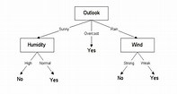
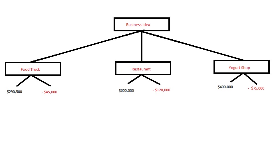
An example of a decision tree is pictured below.
The tree pictured here is designed to help us decide what type of business we should invest our money in: A food truck, a restaurant or a yogurt shop. You can see that based on information obtained from an outside source, we could make $290,500 by investing in a food truck business and we might lose $45,000 if things do not go well. The restaurant business potentially would give us $600,000 in profit if we do well, but poses a significant loss of $128,000. The yogurt shop could earn $400,000 or lose $75,000.
A decision tree can help us determine which of the three investments is the best one. The main idea of decision trees is to find those descriptive features which contain the most information regarding the target feature (type of business to invest in).
Copy and paste the information above into Geany text editor. Here is how the algorithum works.
The expected value is calculated in such a way that it includes all possible outcomes for a decision.
It has been determined by an outside source, if companies that sell this type of information that. (These numbers are approximations only)
Business success and failure rates for a food truck business are 60 pecent and 40 percent.
Business success and failure rates for a restaurant are 52 percent and 48 percent.
Business success and failure rates for a yogurt shop are 50 percent and 50 percent.
We first declare a variable for expected value for each.
Next we multiply the success rate of each by the amount of expected income.
Next we multiply the failure rate by the amount of expected loss.
Now we add these amounts together to come up with our final calculation.
Lastly, we print out the results.
When we execute the program, we can see the results.
Food truck $156,300
Restaurant $254,400
Yogurt shop $162,500
The best investment based our decision tree calculations, would be to invest our money into a restaurant.
Day 4: Decision Tree: Gini Index
Let's suppose that you are a company that sells video games to adult gamers. You want to find out what factors influence the purchases and playing of video games.
You obtain information from a company that sells data and information about purchasing habits and usage of video gamers. You want to examine how age and gender and education affect video gaming time so as to direct your marketing efforts.
An algorithum called the Gini Index is a useful tool to help us decide whether gender, age or education is the biggest influence on playing video games. The Gini Index says, if we select two items from a population at random they must be of the same class,
and the probability for this is 1 if the population is pure. It works with categorical target variable "Success" or Failure". Success equates with playing video games and failure equates with not playing video games. It performs binary splits.
The higher the value of the Gini index the higher homogeneity or the more importance of the variable. The formula is the sum of square of probability for success and failure (p^2 + q^2)
We want to segregate our users based on the target variable (playing video games or not). Here is the information that we will work with.
Our sample size is 300 individuals: 100 females and 200 males.
50 percent play video games.
50 percent of the females play video games.
55 percent of the males play video games
The age groups we are examining are 18-29 year olds and 30-49 year olds.
140 individuals identified themselves as between 18 and 29 years of age.
160 identified themselves as between 30 and 49 years of age.
80 identified themselves as not having a high school diploma.
120 identified themselves as having a high school diploma.
100 said that they had a four year college degree or more.
Put the above code unto the clipboard and then paste it into Geany. Save using a .py extension.
Let us examine the code. The # allows us to make comments about the code. Here is where we show what the variables are.
#Split on gender
female= (0.5)*(0.5) +(0.5)*(0.5)
This line represents the sum of square of probability for success and failure (p^2 + q^2)
The success is the part of the equation represents the number of females in our sample that say that play video games.
The failure part of the equation is the number of females that do not play video games. It is also 50%.
The probabilities are squared (multiplied by each other ) and then added together.
This line equates to .50
female = round(female,4) This line rounds off the variable female to three decimal places.
male = (0.55)*(0.55) + (0.45) * (0.45) This line shows that 55% of the males in our random sample say they play video games. This is the success part of the formula. If 55% saythey play then 45% do not play video games (1.00-.55 = .45)
The result of this line is (.3025 * .2025 = .505)
male = round(male,4) This line rounds off the answer to three decimals
weightedGenderSplit = (100/300)*0.55+(200/300)*0.505 This line produces a weighted average. There 100 females in our study and 200 males. The percentages mentioned in the lines above are multiplied and then added together.
weightedGenderSplit = round(weightedGenderSplit,4) This line rounds off the answer to three decimals
The next lines print the results from the lines above.
print("Age Split") This line prints the title of the next group Age
#age1 - 18-29 year olds This comment line describes the variable age1
#age2 - 30-49 year olds This comment line describes the variable age2
age1 = (0.81) * (0.81) + (0.19) * (0.19). This line contains the algorithm and shows that 81% of the respondents aged 18-29 in our survey indicated that they play video games. Conversly we can calculate that 19% do not play video games.
If you calculate the results of this equation, you wil get .81 *.81 = .6561 + .19 * .19 = .0361 .6561 + .0361 = .6922
age2 = (0.60) * (0.60) + (0.40) * (0.40) This line also contains the algorithm and shows that 60% of 30-49 year olds play video games and 40% do not play.
If you calculate the results of this equation you will get .60 *.60 = .36 = .40 * .40 = .16 .36 + .16 = .52
The next two lines round off the results for age1 and age2
weightedAgeSplit = (140/300) * 0.6922 + (160/300) *(0.52) This line calculates a weighted age split. 140 out of the 300 in the sample stated that they were in age group 18-29
We first calculate the percentage of 18-29 year olds (140 divided by 300) and then multiply by the amount we calculated for age1 split, .6922.
We then calcualte the percentage of 30-49 year olds (160/300) and multiply it by the value obtained for age2 split, 0.52.
Next we add the two results together ( .32 + .27)
Next line rounds off the weightedAgeSplit to three places.
#Education split
Our survey contains three groups based on education level: The first group, were non-high school graduates. Eighty out of our 300 sample indicated that they did not graduate from high school. Forty percent of this group play video games and 60% did not play.
highSchool = (.51) * (.51) + (.49) * (.49) This line is for the high school graduates. One hundred twenty indicated this on the survey and 51% indicated that they played video games while 49% did not play.
collegeGrad = (.57) * (.57) + (.43) * (.43) This line is for those completing 4 or more years of college. One hundred responded that they had a 4-year degree or more and 57% of those play video games.
This line calculates the weightedEducationSplit. Remember 80 were non-grads and .52 of them play video games. 120 were HS grads and 50% of them played video games. There were 100 college grads and .5098 of them played video games.
The next few lines print the results of these calculations.
The final lines compare results and based on the results, a recommended group is displayed (gender, age or education)
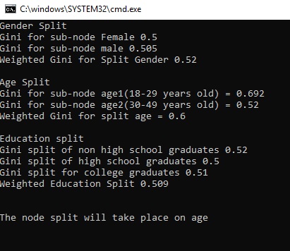
Execute the program. Let's look at the results.
Category
Percentage
Female
0.500
Male
0.505
Weighted Gender
0.52
18-29 year olds
0.6922
20 - 49 year olds
0.52
Weighted Age
0.6004
Non HS grads
0.52
High school grads
0.5002
College grads
0.509
Weighted College grads
0.5086
As you can see the most significant variable of the three is age. The 18-29 year olds play more video games than the older group.
This information can be used to redefine our target market, design video games for this segment of our market, target advertisements and email campaign directed toward this group.
We also found out that gender does not matter that much and neither does the educational level attained by the respondents in the study.
Day 5: Frequent Itemsets via Apriori Algorithm
The market basket analysis approach which uses the frequent Itemsets to find groups of items that occur together frequently in a data set.
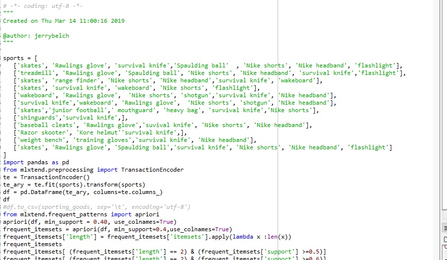
Let's look at an example of a dataset. It is for a sporting goods store. Each line is called an itemset, and represents a sale to an individual.
The name of the dataset is SPORTS. There are total of 12, (0-11) customers. The first customer purchased the following items:skates, Rawlings glove, survival knife, Spaulding ball, Nike shorts, Nike headband, and a flashlight.
The goal is to find the same items in each of the individual sales.
If you look for the same item in each of the 12 sales, you will see that.
Nike shorts were purchased by 9 out of 12 the customer. 9/12 = 75%
Nike headbands were purchased by 8 out of the 12 customers which equals 67%.
Glowman flashlight 4 out of 12 = 33%
Rawlings glove 6 out of 12 = 50%
Skates were purchased by 5 out of the 12 customers equalizng 42%.
Survival knife was a popular item with 83% itemsets in the whole dataset
Spaulding ball purchased by 3 out of the 12 = 25%
We are really most interested in those itemsets over 50% with two or more items in the itemset.
There are some items that represent multiple items purchased by the customers.
Let's look at one itemset that contains 2 different items: Nike shorts and survival knife.
Look at the dataset above. Both items appear for customers 1,2,3,4,5,6,7,and 9.
That is 8 out of 12 or 67% of our customers bought these two items together.
One cannot easily see why a buyer would buy these two items together, but it is certainly worth investigating.
Even knowing just that these two items were purchased together is important. We might want to bundle these two items
together on the shelf or on our web site or offer discounts for this dual purchase.
If we look at the dataset more closely, we can see other dual purchases for multiple customers. Like Nike headbands and Nike shorts, Rawlings glove and Nike headband, Nike shorts and skates, and others.
We could also calculate the number of times each of these transactions occurred to find the percentage. That is a lot of time-consuming work.
With only 12 transactions in the dataset, we can just visually examine it for the information we are looking for.
Suppose our dataset had 10,000 transactions, It could take forever.
That is why we need Python programming language an algorthum and the computer to help us find these relatioships in our customers' data.
The items in each sale are separated by commas. The comma is known as the delimiter. It may be another character such as a semicolon. Each itemset in the whole dataset is enclosed in square brackets. A comma is put at the end of each transaction or row. Comma Separated Value files can be created in any text editor . They can also be created using the save as option in Microsoft
Excel. The entire dataset is enclosed in square brackets. The last row of the data set does not have a comma after the square bracket.
Data mining is a process used by companies to turn raw data into useful information. By using software to look for patterns in large batches of data, businesses can learn more about their customers, develop more effective marketing strategies, increase sales and decrease costs.
There a number of algorithms available to us. We will focus our attention on the Apriori algorithm.
The apriori algorithm has been designed to operate on databases containing transactions, such as purchases by customers of a store. An itemset is considered as "frequent" if it meets a user-specified support threshold. For instance, if the support threshold is set to 0.5 (50%), a frequent itemset is defined as a set of items that occur together in at least 50% of all transactions in the database.
It makes several passes over the dataset, increasing the size of itemsets that are being counted each time. It filters out irrelevant itemsets by using the knowledge gained in the previous passes.
The Apriori algorithm can be downloaded along with many other algorithums in the Anaconda package.
The Apriori algorithum produces the same results as other algorithms. It is quite easy to see that working with only 12 sales and a few items in each sale, that this task is quite simple. Imagine examining 100,000 sales.
What does knowing this information do to help us determine how to better market our products? Knowing what to do with related products is simple. If a customer buys a baseball glove, and a ball you might recommend that they buy a baseball and baseball hat. These associations would be simple to see in a sales transction
What is the association between rink skates and Nike shorts? That is a good question. If we see that there are a large number of these sales, we need to investigate.
We might make the assumption that a baseball pitcher that bought a glove might need a headband to soak up the sweat.