Day 1: Introduction

A convolutional neural network is a type of neural network used to identify images. Each pixel is related to to other pictures. Looking at a single pixel, you can't identify the image, however if you look at many pixels, your can identify the image. That is what a CNN does. It detects features within the image. A combination of these images then forms the complete image, which can be classified with a CNN.

The way a person sees a sketch of a boat.

The boat viewed in pixels.

The way a computer views pixels values 0's and 1's.

Steps in Image Classification

The Convolution Operation
The ReLu Operation
The Pooling Operation
Flattening and Fully Connected Layer

A good source for explaining exactly how these steps work, check out Deep Learning Crash Course for Beginners with Python from AI publishing company.

We will be using the fashion MNIST data set. It contains 60,000 training images and 10,000 test images. Each image is 28 by 28 pixels for a total of 784 pixels.

There are ten classes.

0 T-shirt\top
#1 Trouser
#2 Pullover
#3 Dress
#4 Coat
#5 Sandal
#6 Shirt
#7 Sneaker
#8 Bag
#9 Ankle boot

We are going to create a CNN model that will be able to classify a fashion image into one of the 10 categories.

Day 2: Importing the necessary libraries

We will create a CNN that will be able to classify an image of fashion items such as coats, trousers, sandals into one of 10 predefined categories.

Make sure that you have installed tensorflow.

Open a new Python project, click copy text button and paste the contents into the first frame.

Run the code in the first frame.

This code imports libraries from Python.

Add a new frame, click copy text button and paste the contents into this frame.

Run the code in the first two frames.

This code gets the fashion file and splits the data into training and test sets.

Here is the output from script 2.

x_train shape: (60000, 28, 28, 1)
60000 train samples
10000 test samples

As you can see, the datast contains 60,000 images and the test group contains 10,000 of those images The images and labels are imported here.

The Fashion MNIST dataset is a large freely available database of fashion images that is commonly used for training and testing various machine learning systems. Fashion-MNIST was intended to serve as a replacement for the original MNIST database for benchmarking machine learning algorithms, as it shares the same image size, data format and the structure of training and testing splits.¹

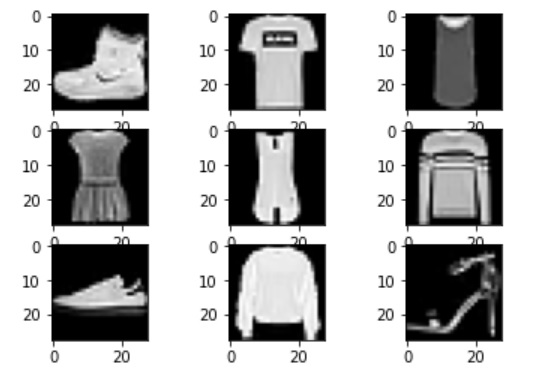
Let's peek inside the dataset. We can visualize some of the items with matplotlib.

Add a new frame, click copy text button and paste the contents into this frame.

Run the code in the first three frames.

This code gets shows images from the test set.

Here is the output from script 2.

These images are 28 by 28 pixels and in greyscale.

Day 3: Individual records and creating the model

Add a new frame, click copy text button and paste the contents into this frame.

Run the code in the first three frames.

This code gets shows you image 2350 in the test set. Try other numbers. Remember that the test set contains 10,000 images with their labels.

Here is the output from script 3.

Add a new frame, click copy text button and paste the contents into this frame.

This script builds the neural network.

Run the code in all the frames. Here is the output

Add a new frame, click copy text button and paste the contents into this frame.

This script trains the neural network.

An epoch is a complete iteration through the entire training dataset in one cycle for training the machine learning model. During an epoch, Every training sample in the dataset is processed by the model, and its weights and biases are updated in accordance with the computed loss or error.

Batch size refers to the number of samples that are propogated through the network.

Run the code in all the frames. Here is the output for the three epochs.

The algorithum is iterative. This means that the search process occurs over a multiple discrete steps, each step hopefully slightly improves the model parameters.

Write down the loss and accuracy numbers for each epoch. Did the loss go down and the accuracy improve with each iteration? That is what you should expect to see.

Day 4: Checking accuracy of the model.

Now we need to see how well our model performed. We will be looking at accuracy and loss. In addition we will check validation accuracy, which is used after the neural network has been trained. It is used to tune the network's hyperparameters. It allows repeatable comparison of these different parameters against the same dataset.

Add a new frame, click copy text button and paste the contents into this frame.

This script prints out the loss and accuracy of the model.

Next we will print the validation loss and validation accuracy.

Add a new frame, click copy text button and paste the contents into this frame.

This script prints out the validation loss and accuracy of the model.

Next we will graph the training and test accuracies.

Add a new frame, click copy text button and paste the contents into this frame.

This script graphs the accuracy and the validation accuracy of the model.

Here is what the output should look like with 3 epochs.

Change the epochs to 20 and run all cells. Your output should look something like this:

Loss	Accuracy	Val_Loss	Val_Accuracy
.5253	.8086	.3656	.8672
.3838	.8620	.3197	.8832
.3437	.8746	.2928	.8942
.3220	.8834	.2849	.8949
.3023	.8893	.2868	.8976
.2950	.8905	.2925	.8933
.2854	.8962	.2670	.9017
.2790	.8991	.2658	.9039
.2703	.9016	.2569	.9078
.2668	.9011	.2614	.9049
.2661	.9038	.2531	.9087
.2541	.9052	.2589	.9053
.2541	.9058	.2559	.9065
.2479	.9095	.2527	.9113
.2502	.9059	.2565	.9068
.2459	.9089	.2630	.9040
.2400	.9119	.2524	.9093
.2393	.9109	.2670	.9042
.2369	.9122	.2555	.9116
.2353	.9127	.2563	.9109

As you can see from the table above, our model with 20 epochs did quite well.

Loss decreased from .52 to .2353.
Validation loss decreased from .3656 to .2563
Accuracy increased from .8086 to .9127
Validation accuracy incresed from .8672 to .9109

Summary of losses and accuracies

Add a new frame, click copy text button and paste the contents into this frame.

This script summarizes the loss and accuracy of the text set.

Here is what the output should look like.

Test loss: 0.2844100892543793
Test accuracy: 0.9004999995231628

Add a new frame, click copy text button and paste the contents into this frame.

This script cisualizes test and training accuracies.

Here is what the output should look like.

Underfitting and Overfitting

Underfitting means that the model did not sufficiently learn the problem and show decreases in loss and increases in accuracy and fails to make accurate predictions.

Overfitting can be described as a model one that makes a correct prediction for every instance in the training set.

Our graph helps us also determine if our model is overfitting. If the training accuracy is higher than the test accuracy it is overfitted. In our case that is not true. Testing accuracy is greater than training accuracy.

We can also see based on the graph, that accuracy improved after each epoch.

Making Predictions

Now we are going to make a prediction on one of the images in the test set. Let's predict the label for image 6789 to see if it is a sneaker, shirt, pants, coat, etc.

Create a new frame and key in the following code.

predictions = model.predict([x_test])
print(np.argmax(predictions[6789]))

Your output should be the number 6, which corresponds to a shirt classification.

Now let's see if image 6789 is really a shirt. Key in the following code in a new frame.

plt.imshow(x_test[6789])
plt.show()

Yes, our model did make a correct prediction. Image 6789 is indeed a shirt, classified as number 6.

Try some other numbers.