Day 3: Creating the Python code to decide type of algorithum to use.
We need to determine what type of model we should construct.
We have assumed that a linear regression model is the right fit.
It is important to know how the relationship between the values of the X axis and the Y axis. We need to see if there is any relationship.
If there is no relationship, we cannot use linear regression as a model.
We believe that there is correation between pay rate and gross profit.
Let's find out.
r = the coefficient of correlation.
r values range from -1 to 1. 0 means no correlation. 1 and -1 means 100% correlated
We have listed the first 20 rates of pay from our dataset on the X axis.
The first 20 amounts of gross pay have been put on the Y axis.
Start a new python project.
Open a new Python project and paste the contents into the the first frame.
Run the code in the first frame.
The r value is 0.9025005300016853 indicating a very positive correlation between rate of pay and gross profit, therefore we can use linear regresssion as our model to make predictions.
We entered 16.35 into our function to predict what gross pay should be with this payrate.
Our model predicted that a pay rate of 16.35 should predict a gross pay of 663.2600816333731. Try entering other pay rates in our model.
One final test: We should graph this data to see if it will produce a straight line, indicating a strong linear relationship.
Day 4: Visualizing the data in our model
Open a new Python project and paste the contents into the the first frame.
Run the code in the first frame.
In the first lines of code we imported matplotlib and scipy.
Next we created an array of the numbers for pay rate from our dataset.
We created another array for the y axis consisting of gross pay.
Next, we executed a method that returns some key values of linear regression.
Now we created a function that uses slope and intercept values that represent where on the y axis the corresponding x value are to be placed.
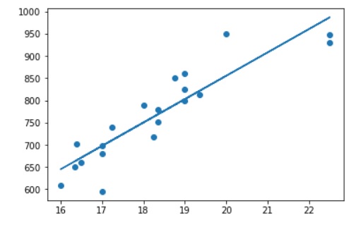
Then we drew the scatterplot.
The line last draws the linear regression line.
Our graph shows a strong relationship between gross pay and rate of pay. We can use a linear regression model to make predictions.
Day 5:Analyzing the payroll using Python linear regression model.
Open a new Python project and paste the contents into the the first frame.
This code imports the libraries needed for this model.
Click on the + to add a new frame.
Paste the code to add the libraries to the project.
Getting and printing the dataset file
Press the + sign to add a new frame.
Paste the code into a new frame.
The dataset represents last month's payroll. It is composed of four weeks. There are 21 employees. In real life, the dataset would be much larger, but we can still see how it works with a much smaller dataset
In this case, the whole dataset is displayed. Normally, with large datasets, the head, which consists of the first 5 lines, is displayed.
The location of the file is up to you. Remember where you saved your dataset file of employees.
You can see the folder that I used is C:\\Users\\jerry\\OneDrive\\Documents\\LinearRegressionAccounting.
Now we are going to put in some code that will describe our dataset.
Describing the dataset
Click on the + to add a new frame.
Paste the clipboard content into the frame.
Splitting the data set into independent variables and dependent variable
Click on the + to add a new frame.
Paste the clipboard content into the frame.
This frame separates the independent variables, (X) from the dependent variable (y).
Click the + key for a new frame and key in: from sklearn.model_selection import train_test_split
Click the + key for a new frame and type: X_train, X_test, y_train, y_test = train_test_split(X,y, test_size= 0.20, random_state=0)
Here is where we begin he process of training the model. We are using a sample size of 20% which results in 17 records. The random state designation makes it so that each time we run the model, the items selected wil be the same.
Click on the + key for a new frame and type: from sklearn.linear_model import LinearRegression
Save your program.
Click on the + and add these two lines in the frame: