Introduction
Before beginning this lesson, you should have previously completed Machine learning Linear Regression
The purpose of this lesson, it for you to do a linear regression analysis on sales calls made for a company that sells portable generators.
Their customers are big-box retailers, hardware stores, recreational vehicle dealerships, contractors, building supply outlets.
We will use Python's linear regression model to accomplish our goals.
We are trying to see the relationship between number of sales calls and the reaulting sales, for our ten sales representatives.
Based on the past year's records of sales calls and number of sales of our generators for the past year for all of our sales reps., we are trying to predict next year sales using liner regression analysis.
Linear regression performs the task to predict a dependent variable value (y) based on a given independent variable (x). So, this regression technique finds out a linear relationship between x (input) and y (output). Hence, the name is Linear Regression.
Linear regression analysis we will attempt to look at the impact of sales calls on number of sales.
Linearity denotes the relationship between two or more variables. If there is a direct relationship, we end up with a graph that shows a straignt line.
The independent variable we will call X and it represents the number of calls made to our customers.
The independent variable will call y and it represents the number of sales made to each customer by our representatives.
On our graph the X axis is the horizontal one and the y axis is the verical axis.
In addition we will learn how to use Jupyter Notebook.
Data Preparation
Our company has ten sales persons:Jerry, Janet, Julie, Shelley, David, Loren, Chris, Kyle, Courtney, and Lynsi. Each one covers five states, so the number of calls differ base on geographical distance between customers.
Some of the contact have been previously established and other are cold calls.
We are going to examine a spreadsheet showing calls and sales for theperiod of twelve months.
Our job is to summarize the data so that it more manageable to work with.
Open the spreadsheet now. Initial spreadsheet
The first column contains the salespersons' id number. The first one starts with 0. Jerry
The second column contains the months of the year for each employee.
The third colum contains the number of calls for each month for each salesperson.
The fourth column contains the number of sales made for each call for each person by the month.
The fifth column contains the revenue generated by each sale: $3,000 per sale.
What you need to add the spreadsheet
The table below summarizes what you need to enter into each cell to give us some totals that we can work with in our Python project to predict sales for the next year.
Cell Formula H1 Total Calls I1 Total Sales H13 =sum(C2:C13) I13 =sum(D2:D13) H25 =sum(C14:C25) I25 =sum(D14:D25) H37 =sum(C26:C37) I37 =sum(D26:D37) H49 =sum(C38:C49) I49 =sum(D38:D49) H61 =sum(C50:C61) I61 =sum(D50:D61) H73 =sum(C62:C73) I73 =sum(D62:D73) H85 =sum(C74:C85) I85 =sum(D74:D85) H97 =sum(C86:C97) I97 =sum(D86:D97) H109 =sum(C98:C109) I109 =sum(D98:D109) H121 =sum(C110:C121) I121 =sum(D110:D121)
Now we will take the totals and create a .csv or comma searated value file.
Open up Notepad. We will create our file here.
First we need the column totals: Call and NumberOfSales.
Case matters in the headings. Capitalize C in calls, the N the O and the S in number of sales.
Next type in the number of calls for salesperson 0 a comma and then the number of sales.
Continue in the same fashion for the rest of the sales force. Your file should look like this.
Calls,NumberOfSales
1155,2310
1188,2357
1179,2370
1178,2171
952,1915
911,1863
1168,2382
1190,2380
1000,2000
989,1988
Save your file in This PC, Windows(C:) Users and your user name. Call it SC.csv.
This file location is the one that is accessed by Python.
This information is in the article section of the web page
Jupyter Notebook info
Jupyter Notebook (formerly IPython Notebooks) is a web-based interactive computational environment for creating Jupyter notebook documents. The "notebook" term can colloquially make reference to many different entities, mainly the Jupyter web application, Jupyter Python web server, or Jupyter document format depending on context. A Jupyter Notebook document is a JSON document, following a versioned schema, and containing an ordered list of input/output cells which can contain code, text (using Markdown), mathematics, plots and rich media, usually ending with the ".ipynb" extension.
A Jupyter Notebook can be converted to a number of open standard output formats (HTML, presentation slides, LaTeX, PDF, ReStructuredText, Markdown, Python) through "Download As" in the web interface, via the nbconvert library or "jupyter nbconvert" command line interface in a shell. To simplify visualisation of Jupyter notebook documents on the web, the nbconvert library is provided as a service through NbViewer which can take a URL to any publicly available notebook document, convert it to HTML on the fly and display it to the user. (Wikipedia)
Make certain that Anaconda is installed. The Jupyter Notebook is part of the installation along with all of Python's libraries.
Please follow the steps below in order to Install Anaconda in windows:
Search Anaconda on Google. Click on the official link.
Select the appropriate OS.
Choose the version and bit according to your requirements.
Go the download path after the download is complete.
Double Click on the executable file to begin the installation process.
How to Run Jupyter Notebook with Anaconda Installed.
Click on Start button Select Anaconda from the programs
Click on Jupyter Notebook
The kernel loads first. Click on the link below to learn more about the kernel.
Right after the kernel runs, Jupyter notebook is executed.
Your screen should look like the image below.
Kernel definition
Your screen should look like the image above.
Roll over the image to enlarge it.
Key this code in the first box.
You may copy and paste if you wish.
Below is the file you will need.
Save it in MyPc Windows C drive and your user name.
There are number ways to test or run your code.
Click Run on the menu bar to run all lines of code.
Click the
⇥ To the left of the box to run just this cell.
The output from the cell appears just below.
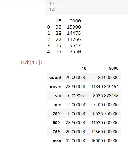
The first five lines of the dataset are displayed. This is called the head.
The dataset is then described. It shows the mean of both variables, the standard deviation, high and low, etc"
Click on Insert and then insert cell below to get a new cell.
You can see from the graph, that it plots an almost straight line, which means that there is a direct correlation between number of hits to the web site and the revenue that is generated.
Now we need to subdivide the data into attributes and labels. The attributes are the independent variables, the hits on the web site, and labels are the dependent variables, revenue generated.
We are trying to predict revenue based on hits.
X = dataset.iloc[:, :-1].values
Y = dataset.iloc[:, 1].values
The X variable will store the attributes, the hits.
The Y variable will store the labels, the revenue generated.
Now we need to divide our data into two sets:training and test.
The Scikit-Learn library lets us do this.
Add these nine lines to the cell we just created.
Save your work by clicking the save icon.
Now run this cell to get the intercept and the coeffient.
What this means that for every additional hit, revenue will increase by $500.
Now it is time to make predictions based on the data we preserved as the training set.
Add these lines below to a new cell in Jupyter Notebook.
The results of printing the dataframe, appear below.
Actual PredictedThe program selected at random six actual values from the entire list.
If you look at the actual list you will see that 14475 was number 2 on the list. Remember count starting with zero.
14475 was #2
14550 was #16
10059 was #14
1055 was #17
7500 was #5
1600 was #4
The random_state code makes it give the same results each time you execute the program.
Remove that part of the line.
Run the code for the last two cells
You should get different results each time for the actual ones selected and the predictions.
Look how close the predictions are to the actual numbers.
The algorithum did an excellent job.
Editing files using Jupyter
You can create and edit files using Jupyter Notebook.
It has the capabilities of any text editor.
It very useful when working with .csv files
Just Click on File and Open
The comma separated value file
Calls,NumberOfSalesYou should have already created a .csv file using notebook.
Make sure that you called the file sc.csv
Save the file in the Windows Users, your name directory.
How to code the sales calls application
Run Jupyter notebook using Anaconda from your start menu.
Start a new file.
Copy the code below and paste it into the first cell of the notebook.
Save and test.
Copy the text below and paste it into the second cell of the Jupyter Notebook.
Save and run.
Your results should look like the image below.
As you can see from the image the results are printed by the head and tail ends of the data.
There are only ten items in the file, so all data is printed. The head and tail function each print five items.
The describe function provides us with a lot of information about the performance of our sales force.
The count 10 salespersons
The mean 1081 for calls 2174 for sales
Standard Deviation 108 for calls and 213 for sales
Minimum calls 911 and minimum sales 1883
Maximum calls 1190 and 2382 for sales
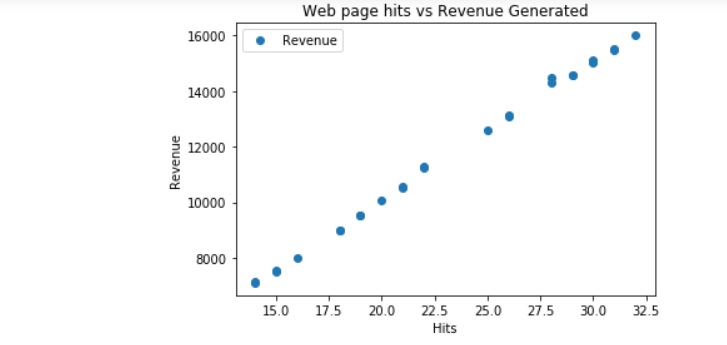
The code above graphs the information contained in the file.
Calls are on the x axis.
Number of Sales are on the Y axis.
As you can see by the visualization of the data, that there is definite linear relationship between the number of calls made and the resulting number of sales.
The first two line of code in this cell involves subdividing the data into attributes, the independent variable, calls and the labels, number of sales, the dependent variable.
The first two lines extract the data. The X variable will store the calls and the y variable the number of sales.
We now need to divide the data into two sets:training and test.
The test set will learn from the training data.
The Scikit-Learn library gives us the method we need to accomplish this split.
Twenty percent will be the size of the test group and eighty percent will comprise the training data set.
Our dataset is small, only 10 items. But remember that it summarizes many calls and sales for the entire year.
Consequently, the test group only contains two items.
The random_state=0 code makes it so that when you run the program, the same items are picked at randonm each time.
If you remove the randon_state code, each run will produce different examples.
The code in the cell above does not produce any output. It just processes the data.
The fit() method passes the training data.
We have alread calculated the intercept, which is the slope of the line.
The value of the slope is shown by the coefficient.
This linear-regressor coefficient is a very helpful number in our analysis of calls and sales.
It tells us that if each sales person makes an additional one call per month that the number of sales for each will increase by almost two generators sold.
Predictions
We can now use the training set to make some predictions.
Add these three lines at the end of your existing code.
pred_y = linear_regressor.predict(X_test)
We only see two actual and predicted cases, since our test set only contains 20% of a total of ten.
The model is pretty close to the actual sales.
Two cases were selected at random. They are actual sales of 2370 and 2000.
The predicted sales are 2365.52 and 2019.55.
If we make a slight adjustment to the code relating to the random_state, we will get different results, each time we execute the code in couple of cells.
Delete the code involving ",random_state=0".
Save and run code. You should get different actual and prediction numbers each time you execute the code.
I did this and the following spreadsheet gives the results that I got.
Spreadsheet of actual and predictions.
Initial raw data
Get the following file "SalesCalls3.csv" listed below.
Change the csv file name to "salesCalls3.csv"
Run the program. Remember to start at the second cell, where the code retrieves the file.
After using linear regression and Python to predict sales, what conclusions can you make about the model using the different files?
What recommendations should the sales manager make to their sales staff?
Accuracy of the predictions
There three regression algorithums for linear regression problems.
MAE (Mean Absolute Error)
MSE(Mead Square Error)
RMSE(Root Mean Squared Error)
Example on how the evaluation accuracy metrics work
I will use the Mean Absolute Error, since that is the easiest one to explain.
Let's assume that the following information.
Original or actual data is: 234, 260,269,262
The predicted data is: 231,254,260,257
First find the difference between original and predicted amounts.
Subtract 231 from 234.
Subtract 254 from 260.
Subtract 260 from 269.
Subtract 257 from 262.
Add the differences up: 3,6,9,5 = 23
Divide 23 by 4, the number of items to get the average.
Answer is 5.75
The most important for linear regression problems is RMSE (Root Mean Squared Error).
RMSE measures the vertical distance between the point to the line.
Root mean squared error (RMSE): RMSE is a quadratic scoring rule that also measures the average magnitude of the error.
It’s the square root of the average squared differences between prediction and actual observation.
A zero score never happens. A zero score would be a perfect fit for the data and the regresssion line.
The lower the RMSE the better.
Copy the code above and paste it into the Jupyter editor at the end of your code.
Save and Run.
Multiple Linear Regression
This next assignment has to do with evaluating the effectiviness of different advertising campaigns.
There has been a prominent trend in media choice for advertising expenditures. In the past, the expenditures focused on traditional media types: television, radio, newspapers, magazines, point of sale, direct mail, etc.
Nowadays, there has been a shift toward digital media: email, Facebook, InstaGramp, Twitter, web pages, search engines advertising.
Your small business sells athletic leisure wear. Their target market is the Millennial generation. They have a $10,000 monthly budget for advertising. The money is allocated to each of the following media types.
Digital media - 32.9%
Television - 38.7%
Radio - 9.1%
Newspapers - 10.4%
Magazines - 8.8%
The company wants to see what factor has the most important influence on revenue.
They decide to look at type of media, money spent on advertisng and return on investment.
Return on investment is calculated as follows: Roi = (Net Profit/Cost). For example, if your revenue for an advertsing campaign was $3,700 and you spent $3,000 on advertsing, then your roi would be (4000-3000)/3000 or .23333.
The file shows information for six months for each of the media types.
Digital is assigned the number 1
TV is assigned number 2
Raido is assigned number 3
Newspapers are assigned number 4
Magazines are assigned number 5
Revenue was calcuated fore each campaign.
The file was developed using the comma separated value style.
Copy the text on the clipboard and save it to Windows drive C:, Users, and your name as the user.
Call the file adSales.csv
For the first two months, the amount spend on advertising remained the same. Of course, revenue and roi differed slightly.
In March, the company decided spend 10% less on all advertsing media amounts.
In April, the company decided to increase the amount spend on digital media and keep the same expenditures for the rest of the media types.
In May, they decided to reduce spending on all non-digital media by 15% and increase their digital presence by 15%.
In June they continued with the same strategy as in the month of May.
They have decided to use a multiple regression Python model to test the effectiviness of their advertisng campaign.The steps involved in developing the model are almost identical to the ones in developing a Linear regression model with only two variables.
The difference in the two models comes when they make an evaluation.
We need to know which factor: media type, amount spent or roi have the most influence on revenue.
We are going to use Jupyter Notebook as our text editor.
Here is the code.
Copy the code and paste it into Jupyter Notebook.
Run the code and answer the following questions.
The describe function provides us with some valuable information. Answer the following questions
What is the mean amount spent?
What is the mean for roi?
What is the minimum amount?
What is the maximum amount?
Looking at the first graph, is there a linear relationship between amount spent and revenue generated?
Looking at the second graph, does a linear realtionship exist between roi and revenue?
What are the different coefficients?
Which factor most influences the amount of revenue?